Tree-based models
Decision Trees
Decision trees [1] are popular nonparametric models that iteratively split a training dataset into smaller, more homogenous subsets. Each node in the tree is associated with a decision rule, which dictates how to divide the data the node inherits from its parent among each of its children. Each leaf node is associated with at least one data point from the original training set.
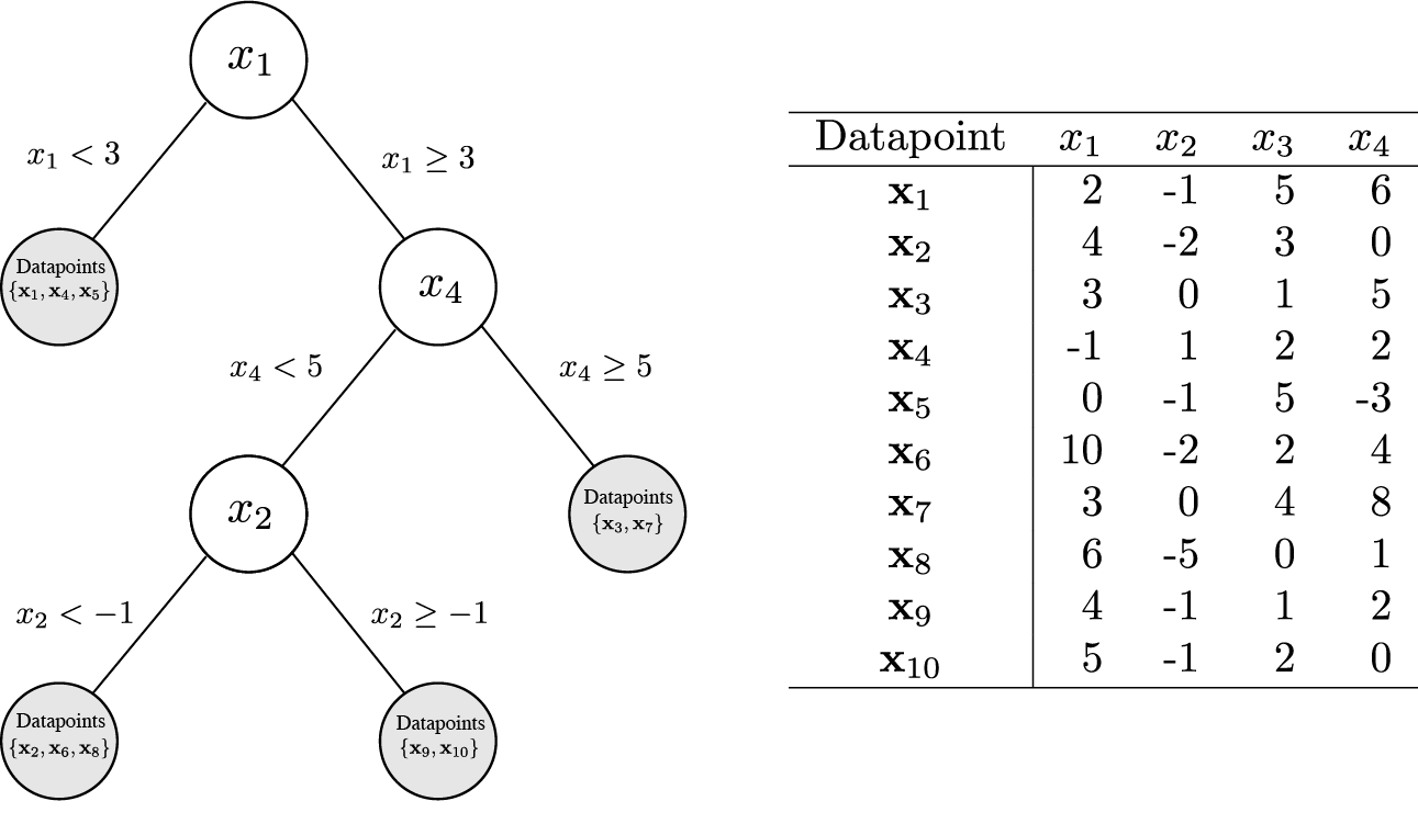
A binary decision tree trained on the dataset \(X = \{ \mathbf{x}_1, \ldots, \mathbf{x}_{10} \}\). Each example in the dataset is a 4-dimensional vector of real-valued features labeled \(x_1, \ldots, x_4\). Unshaded circles correspond to internal decision nodes, while shaded circles correspond to leaf nodes. Each leaf node is associated with a subset of the examples in X, selected based on the decision rules along the path from root to leaf.
At test time, new examples travel from the tree root to one of the leaves, their path through the tree determined by the decision rules at each of the nodes it visits. When a test example arrives at a leaf node, the targets for the training examples at that leaf node are used to compute the model’s prediction.
Training decision trees corresponds to learning the set of decision rules to partition the training data. This learning process proceeds greedily by selecting the decision rule at each node that results in the greatest reduction in an inhomogeneity or “impurity” metric, \(\mathcal{L}\). One popular metric is the information entropy:
where \(P_n(\omega_j)\) is the fraction of data points at split n that are associated with category \(\omega_j\). Another useful metric is the Gini impurity:
For a binary tree (where each node has only two children), the reduction in impurity after a particular split is
where \(\mathcal{L}(x)\) is the impurity of the dataset at node x, and \(P_{\text{left}}\)/\(P_{\text{right}}\) are the proportion of examples at the current node that are partitioned into the left / right children, respectively, by the proposed split.
Models
References
| [1] | Breiman, L., Friedman, J. H., Olshen, R. A., and Stone, C. J. (1984). Classification and regression trees. Monterey, CA: Wadsworth & Brooks/Cole Advanced Books & Software. |
Bootstrap Aggregating
Bootstrap aggregating (bagging) methods [2] are an ensembling approach that proceeds by creating n bootstrapped samples of a training dataset by sampling from it with replacement. A separate learner is fit on each of the n bootstrapped datasets, with the final bootstrap aggregated model prediction corresponding to the average (or majority vote, for classifiers) across each of the n learners’ predictions for a given datapoint.
The random forest model [3] [4] is a canonical example of bootstrap aggregating. For this approach, each of the n learners is a different decision tree. In addition to training each decision tree on a different bootstrapped dataset, random forests employ a random subspace approach [5]: each decision tree is trained on a subsample (without replacement) of the full collection of dataset features.
Models
References
| [2] | Breiman, L. (1994). “Bagging predictors”. Technical Report 421. Statistics Department, UC Berkeley. |
| [3] | Ho, T. K. (1995). “Random decision forests”. Proceedings of the Third International Conference on Document Analysis and Recognition, 1: 278-282. |
| [4] | Breiman, L. (2001). “Random forests”. Machine Learning. 45(1): 5-32. |
| [5] | Ho, T. K. (1998). “The random subspace method for constructing decision forests”. IEEE Transactions on Pattern Analysis and Machine Intelligence. 20(8): 832-844. |
Gradient Boosting
Gradient boosting [6] [7] [8] is another popular ensembling technique that proceeds by iteratively fitting a sequence of m weak learners such that:
where b is a fixed initial estimate for the targets, \(\eta\) is a learning rate parameter, and \(w_{i}\) and \(g_{i}\) denote the weights and predictions of the \(i^{th}\) learner.
At each training iteration a new weak learner is fit to predict the negative gradient of the loss with respect to the previous prediction, \(\nabla_{f_{i-1}} \mathcal{L}(y, \ f_{i-1}(X))\). We then use the element-wise product of the predictions of this weak learner, \(g_i\), with a weight, \(w_i\), computed via, e.g., line-search on the objective \(w_i = \arg \min_{w} \sum_{j=1}^n \mathcal{L}(y_j, f_{i-1}(x_j) + w g_i)\) , to adjust the predictions of the model from the previous iteration, \(f_{i-1}(X)\):
The current module implements gradient boosting using decision trees as the weak learners.
Models
References
| [6] | Breiman, L. (1997). “Arcing the edge”. Technical Report 486. Statistics Department, UC Berkeley. |
| [7] | Friedman, J. H. (1999). “Greedy function approximation: A gradient boosting machine”. IMS 1999 Reitz Lecture. |
| [8] | Mason, L., Baxter, J., Bartlett, P. L., Frean, M. (1999). “Boosting algorithms as gradient descent” Advances in Neural Information Processing Systems, 12: 512–518. |